Using Self-Organizing Maps with SOMbrero for dissimilarity matrices
07 octobre, 2025
Source:vignettes/e-doc-relationalSOM.Rmd
e-doc-relationalSOM.RmdBasic package description
SOMbrero implements different variants of the
Self-Organizing Map algorithm (also called Kohonen’s algorithm). To
process a given dataset with the SOM algorithm, you can use the function
trainSOM().
This documentation only considers the case of dissimilarity matrices.
Arguments
The trainSOM function has several arguments, but only
the first one is required. This argument is x.data which is
the dataset used to train the SOM. In this documentation, it is passed
to the function as a square matrix or data frame, which entries are
dissimilarity measures between pairs of observations. The diagonal of
this matrix must contain only zeros.
The other arguments are the same as the arguments passed to the
initSOM function (they are parameters defining the
algorithm, see help(initSOM) for further details).
Outputs
The trainSOM function returns an object of class
somRes (see help(trainSOM) for further details
on this class).
Graphics
The following table indicates which graphics are available for a relational SOM.
| What SOM or SC Type |
SOM Energy |
Obs |
Prototypes |
Add |
SuperCluster (no what) |
Obs |
Prototypes |
Add |
|---|---|---|---|---|---|---|---|---|
| (no type) | x | |||||||
| hitmap | x | x | ||||||
| color | x | |||||||
| lines | x | x | x | x | ||||
| meanline | x | x | ||||||
| barplot | x | x | x | x | ||||
| pie | x | x | ||||||
| boxplot | x | x | ||||||
| poly.dist | x | x | ||||||
| umatrix | x | |||||||
| smooth.dist | x | |||||||
| mds | x | x | ||||||
| grid.dist | x | |||||||
| words | x | |||||||
| names | x | x | x | |||||
| graph | x | x | ||||||
| projgraph | x | x | ||||||
| grid | x | |||||||
| dendrogram | x | |||||||
| dendro3d | x |
Case study: the lesmis data set
The lesmis data set is based on the co-appearance graph
of the characters of the novel Les Misérables (Victor Hugo). Each vertex
stands for a character whose name is given by the vertex label. One edge
means that the corresponding two characters appear in a common chapter
in the book. Each edge also has a value indicating the number of
co-appearances. The co-appearance network has been extracted by D.E.
Knuth (1993).
The lesmis data contain two objects: the first
one,lesmis, is an igraph object (see the igraph web page), with 77 nodes and
254 edges.
Further information on this data set is provided with
help(lesmis).
data(lesmis)
lesmis
## This graph was created by an old(er) igraph version.
## ℹ Call `igraph::upgrade_graph()` on it to use with the current igraph version.
## For now we convert it on the fly...## IGRAPH 3babff7 U--- 77 254 --
## + attr: layout (g/n), id (v/n), label (v/c), value (e/n)
## + edges from 3babff7:
## [1] 1-- 2 1-- 3 1-- 4 3-- 4 1-- 5 1-- 6 1-- 7 1-- 8 1-- 9 1--10
## [11] 11--12 4--12 3--12 1--12 12--13 12--14 12--15 12--16 17--18 17--19
## [21] 18--19 17--20 18--20 19--20 17--21 18--21 19--21 20--21 17--22 18--22
## [31] 19--22 20--22 21--22 17--23 18--23 19--23 20--23 21--23 22--23 17--24
## [41] 18--24 19--24 20--24 21--24 22--24 23--24 13--24 12--24 24--25 12--25
## [51] 25--26 24--26 12--26 25--27 12--27 17--27 26--27 12--28 24--28 26--28
## [61] 25--28 27--28 12--29 28--29 24--30 28--30 12--30 24--31 31--32 12--32
## [71] 24--32 28--32 12--33 12--34 28--34 12--35 30--35 12--36 35--36 30--36
## + ... omitted several edges
plot(lesmis, vertex.size = 0)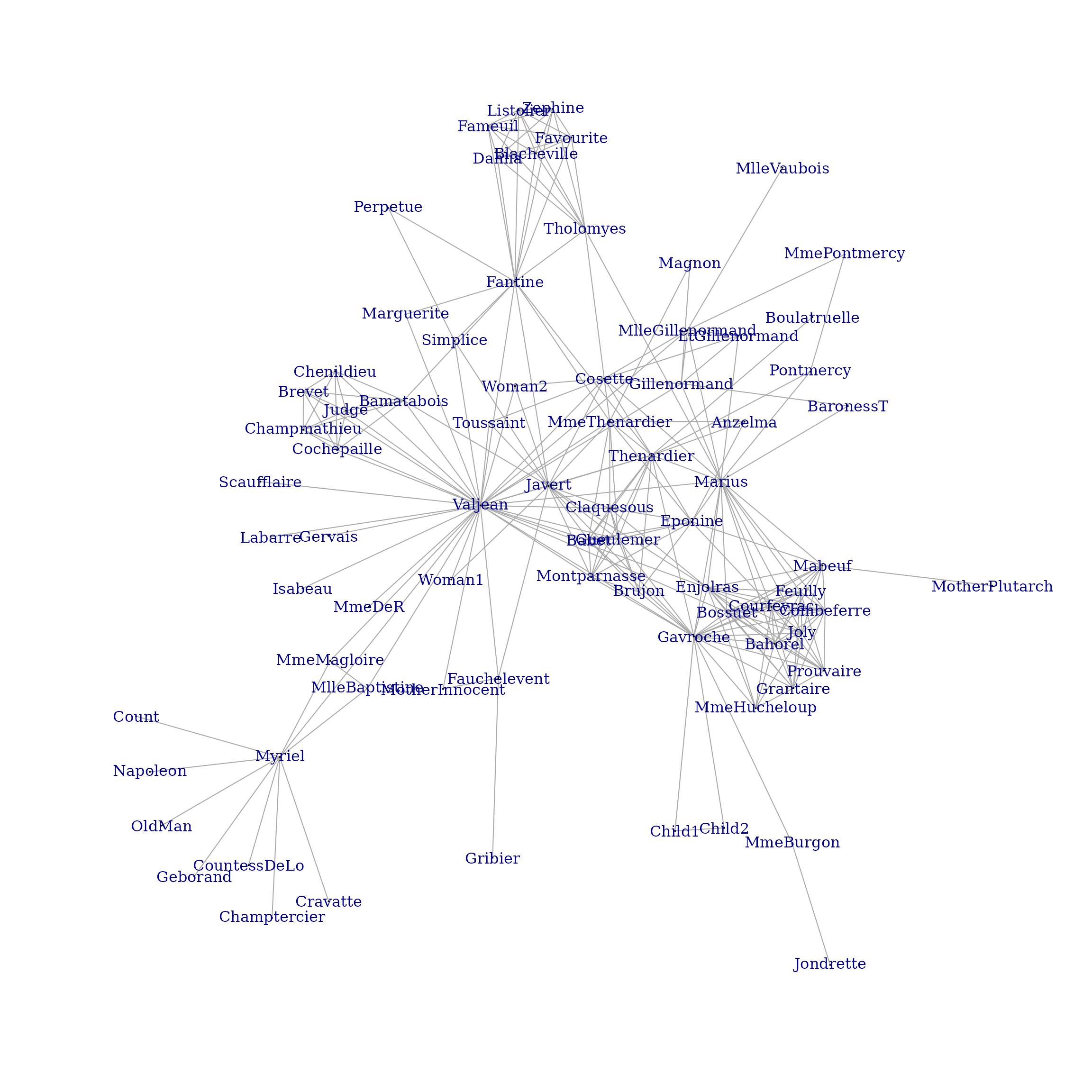
The dissim.lesmis object is a matrix with entries equal
to the length of the shortest path between two characters (obtained with
the function shortest.paths of package
igraph). Note that its row and column names have been
initialized with the characters’ names to ease the use of the graphical
functions of SOMbrero.
Training the SOM
set.seed(622)
mis.som <- trainSOM(x.data=dissim.lesmis, type = "relational", nb.save = 10,
                   init.proto = "random", radius.type = "letremy")
plot(mis.som, what="energy")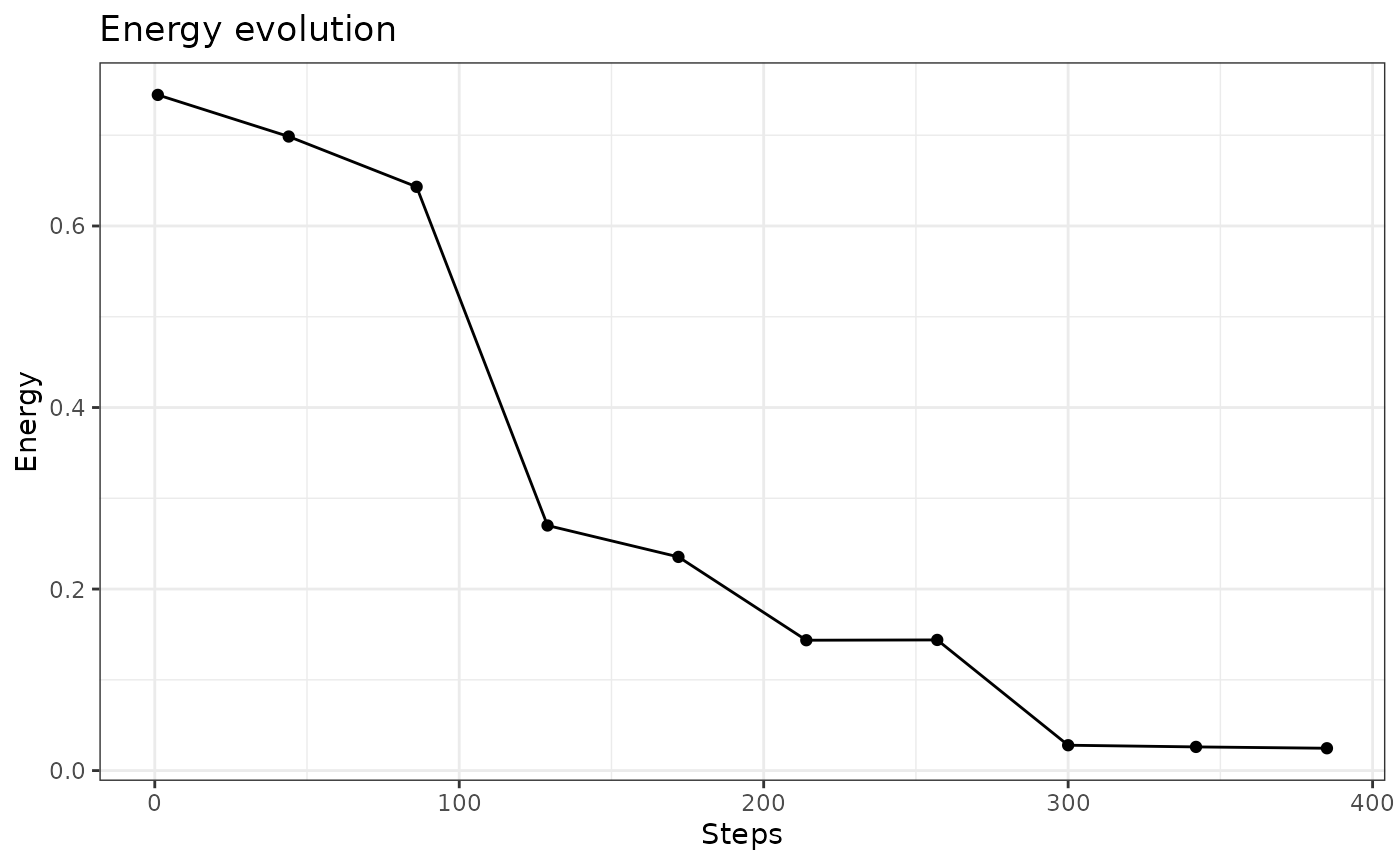
The dissimilarity matrix dissim.lesmis is passed to the
trainSOM function as input. As the SOM intermediate backups
have been registered (nb.save = 10), the energy evolution
can be plotted: it stabilized in the last 100 iterations.
Resulting clustering
The clustering component provides the classification of each of the
77 characters. The table function is a simple way to view
data distribution on the map.
mis.som$clustering## Myriel Napoleon MlleBaptistine MmeMagloire
## 25 25 19 19
## CountessDeLo Geborand Champtercier Cravatte
## 25 25 25 25
## Count OldMan Labarre Valjean
## 25 25 22 22
## Marguerite MmeDeR Isabeau Gervais
## 16 22 23 23
## Tholomyes Listolier Fameuil Blacheville
## 11 11 11 11
## Favourite Dahlia Zephine Fantine
## 11 11 11 11
## MmeThenardier Thenardier Cosette Javert
## 2 6 7 17
## Fauchelevent Bamatabois Perpetue Simplice
## 18 21 11 17
## Scaufflaire Woman1 Judge Champmathieu
## 22 22 21 21
## Brevet Chenildieu Cochepaille Pontmercy
## 21 21 21 9
## Boulatruelle Eponine Anzelma Woman2
## 6 1 2 17
## MotherInnocent Gribier Jondrette MmeBurgon
## 18 18 15 15
## Gavroche Gillenormand Magnon MlleGillenormand
## 15 3 3 13
## MmePontmercy MlleVaubois LtGillenormand Marius
## 8 13 8 4
## BaronessT Mabeuf Enjolras Combeferre
## 3 5 10 5
## Prouvaire Feuilly Courfeyrac Bahorel
## 10 5 5 10
## Bossuet Joly Grantaire MotherPlutarch
## 10 10 10 5
## Gueulemer Babet Claquesous Montparnasse
## 1 1 1 1
## Toussaint Child1 Child2 Brujon
## 17 15 15 1
## MmeHucheloup
## 10
table(mis.som$clustering)##
## 1 2 3 4 5 6 7 8 9 10 11 13 15 16 17 18 19 21 22 23 25
## 6 2 3 1 5 2 1 2 1 7 9 2 5 1 4 3 2 6 5 2 8
plot(mis.som)
The clustering can be displayed using the plot function
with type = names.
plot(mis.som, what = "obs", type = "names")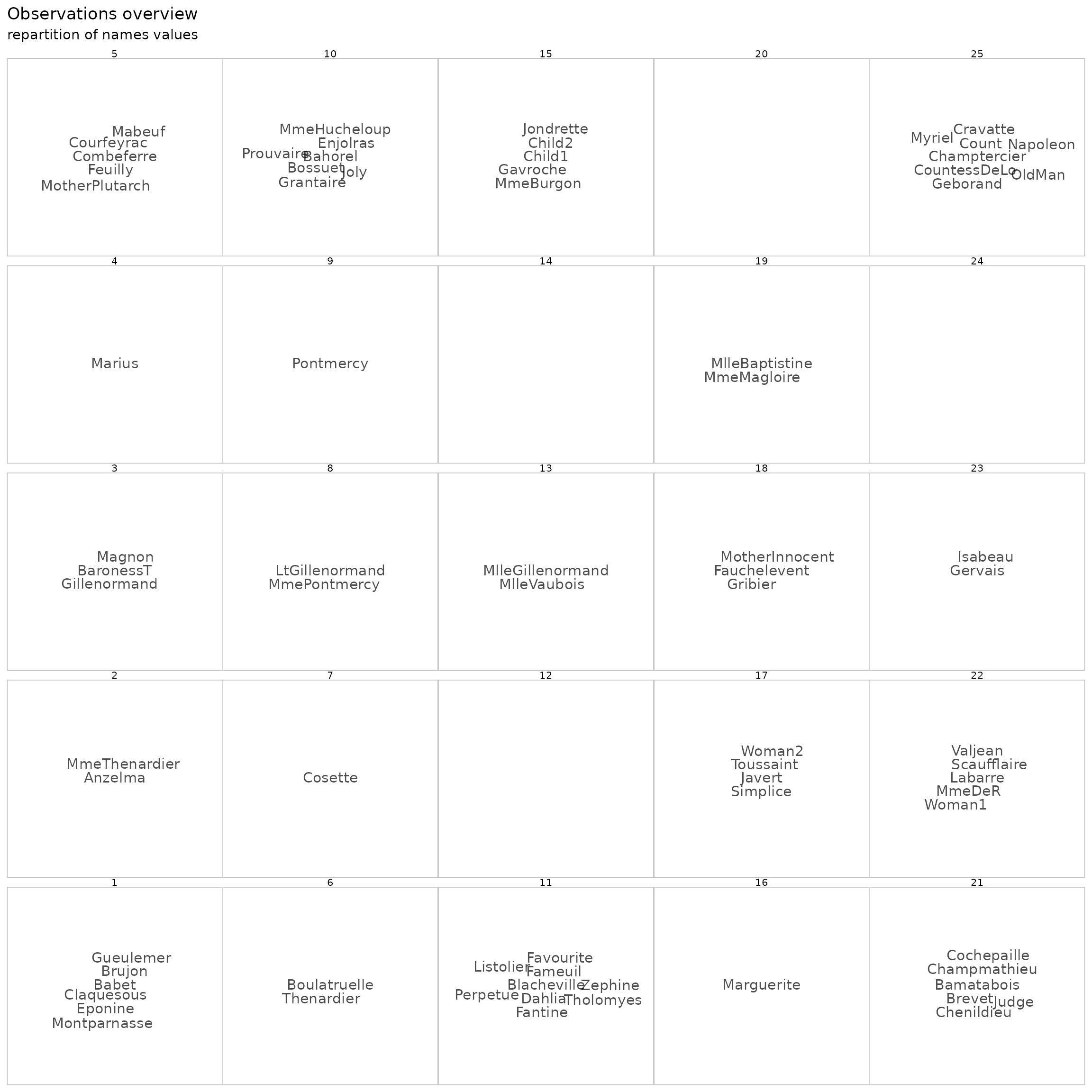
In this clustering, the main character, Valjean, is in a central position (in cluster 8) and some clusters are easily identified as sub-stories around Javert. For instance, clusters 10, 15 and 20 are related to the Thénardier family, with (for instance), cluster 20 being the cluster of Gavroche and his two brothers (named children 1 and 2).
The original graph can also be superimposed on the map:
plot(mis.som, what = "add", type = "graph", var = lesmis)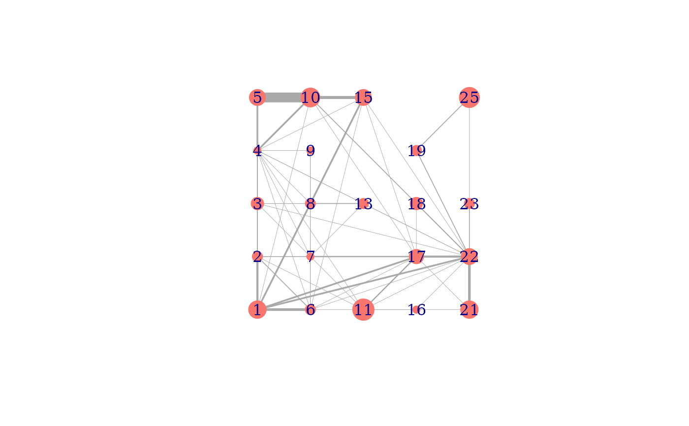
In the latter plot (which is still messy at this stage of the analysis), nodes correspond to clusters and are positioned at the cluster location on the map. The size of the nodes is proportional to the number of characters classified in this cluster and edges between nodes have a width proportional to the total weight between any two characters from the two linked clusters.
Clusters profile overviews can be plotted either with e.g.,
lines or barplot, that both provide an information similar to that given
by "names".
plot(mis.som, what = "prototypes", type = "lines")  +
  guides(color = guide_legend(keyheight = 0.5, ncol = 2, label.theme = element_text(size = 6))) +
  theme(axis.text.x = element_blank(), axis.ticks.x = element_blank())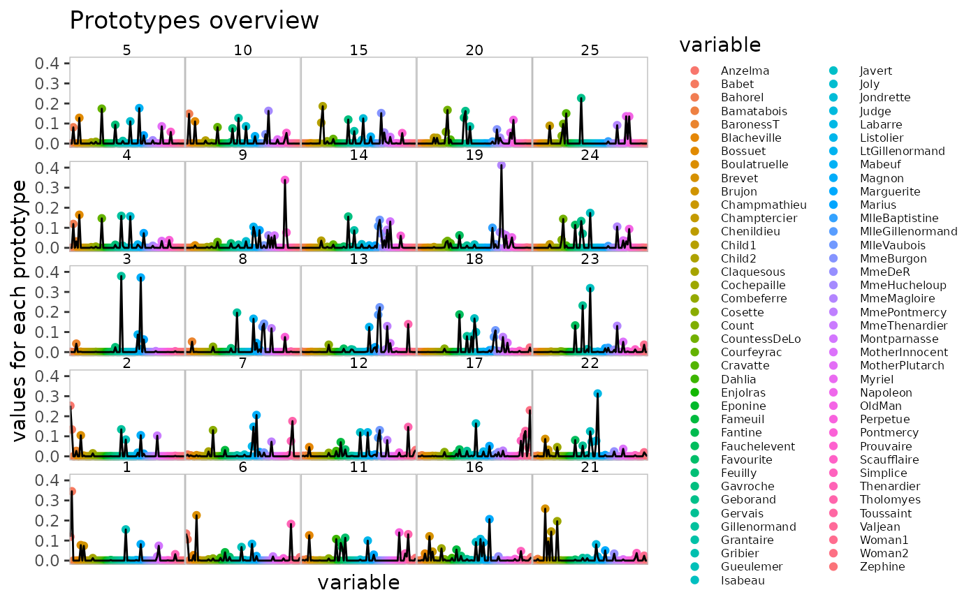
plot(mis.som, what = "prototypes", type = "barplot")  +
  guides(fill = guide_legend(keyheight = 0.5, ncol = 2, label.theme = element_text(size = 6))) +
  theme(axis.text.x = element_blank(), axis.ticks.x = element_blank())
On these graphics, one variable is represented respectively with a point or a slice. It is therefore easy to see which variable affects which cluster.
To see how different the clusters are, some graphics show the
distances between prototypes. These graphics have exactly the same
interpretation as for the other data types processed by
SOMbrero.
"poly.dist"represents the distances between neighboring prototypes with polygons plotted for each cell of the grid. The smaller the distance between a polygon’s vertex and a cell border, the closer the pair of prototypes. The colors encode the number of observations in the neuron;"umatrix"fills the neurons of the grid using colors that represent the average distance between the current prototype and its neighbors;"smooth.dist"plots the mean distance between the current prototype and its neighbors with a color gradation;"mds"plots the number of the neuron on a map according to a Multi-Dimensional Scaling (MDS) projection;"grid.dist"plots a point for each pair of prototypes, with the coordinates representing the distance between the prototypes in the input space, and coordinates representing the distance between the corresponding neurons on the grid.
plot(mis.som, what = "prototypes", type = "poly.dist")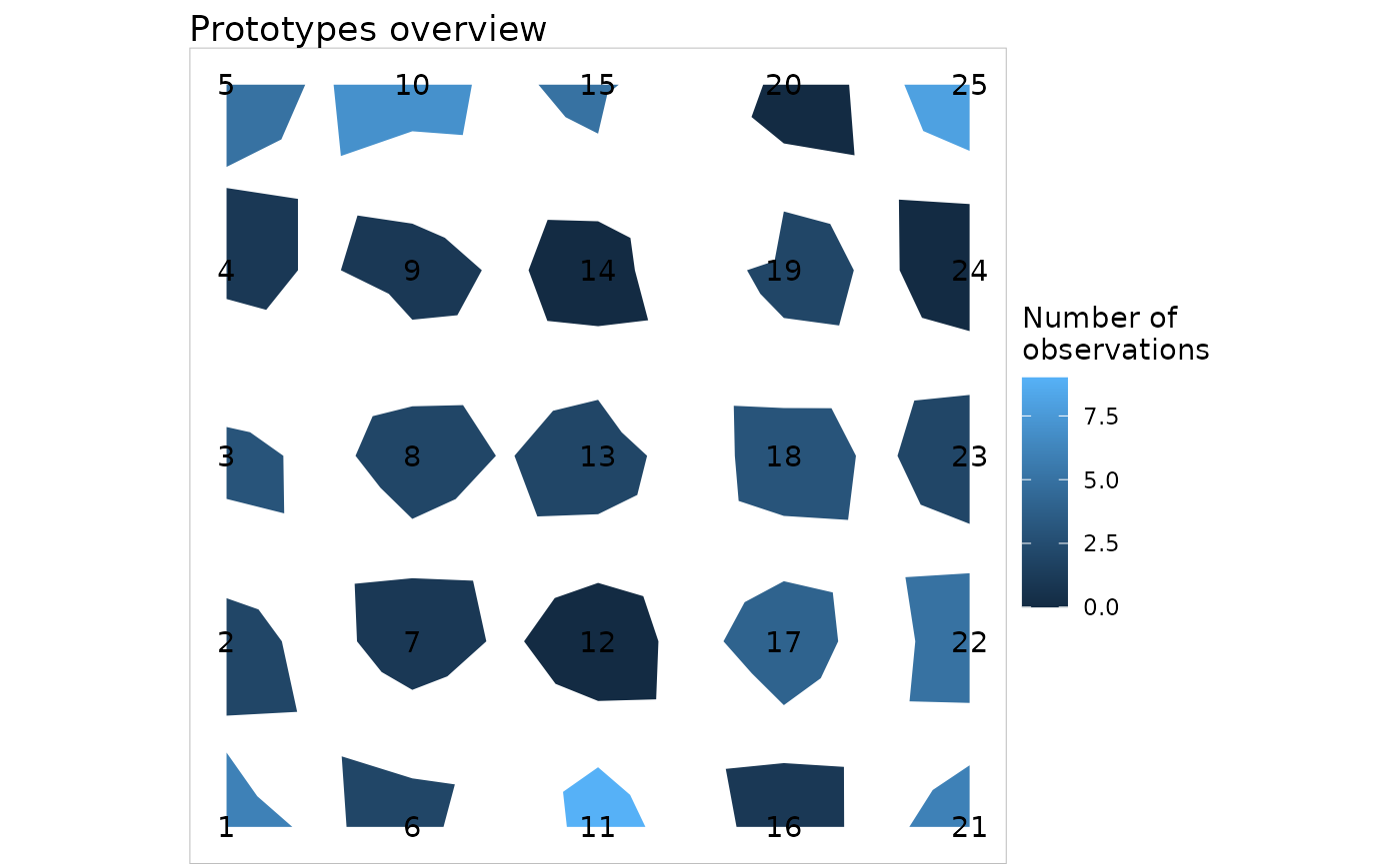
plot(mis.som, what = "prototypes", type = "smooth.dist")
plot(mis.som, what = "prototypes", type = "umatrix")
plot(mis.som, what = "prototypes", type = "mds")
plot(mis.som, what = "prototypes", type = "grid.dist")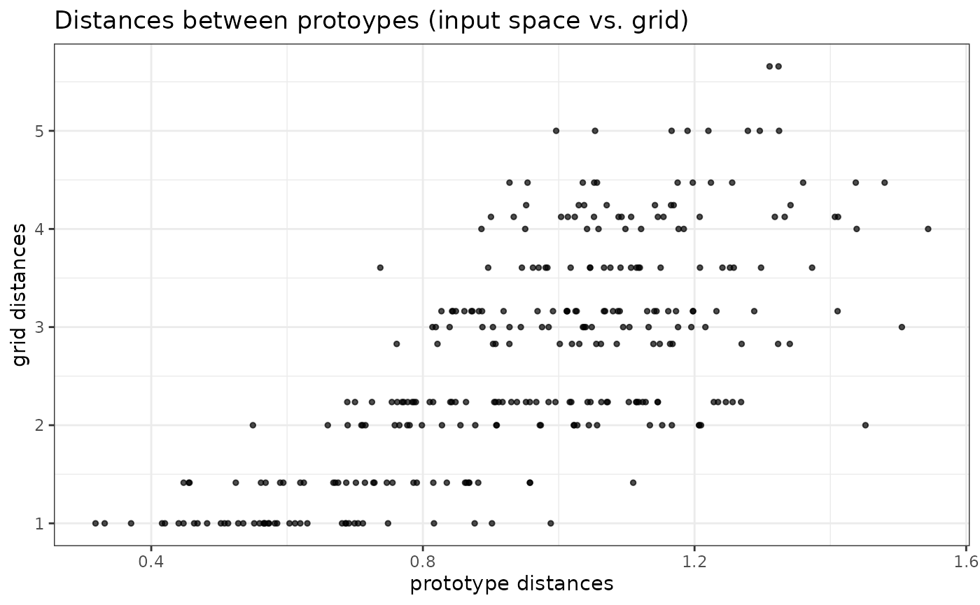
Here we can see that the prototypes located in the top left and top right corners of the map (e.g., clusters 5 and clusters 19-20 and 24-25) are further from the other neurons than in average.
Finally, with a graphical overview of the clustering
plot(lesmis, vertex.label.color = rainbow(25)[mis.som$clustering],
     vertex.size = 0)
legend(x = "left", legend = 1:25, col = rainbow(25), pch = 19)
We can see that (for instance) cluster 25 is very relevant to the
story: as the characters of this cluster appear only in the sub-story of
the Bishop Myriel, he is the only connection for all other
characters of cluster 25. The same kind of conclusion holds for cluster
20 (with Gavroche), among others. Most of the other clusters have a
small number of observations: it thus seems relevant to compute super
clusters.
Compute super clusters
As the number of clusters is rather large with the SOM algorithm, it is possible to perform a hierarchical clustering on top of SOM results. First, let us have an overview of the dendrogram:
plot(superClass(mis.som))
## Warning in plot.somSC(superClass(mis.som)): Impossible to plot the rectangles: no super clusters.According to the proportion of variance explained by super clusters, 5 groups seem to be a good choice (4 groups would have been relevant also. The clustering with 5 groups creates a group with only one cluster in it).
sc.mis <- superClass(mis.som, k = 5)
summary(sc.mis)
##
## SOM Super Classes
## Initial number of clusters: 25
## Number of super clusters : 5
##
##
## Frequency table
## 1 2 3 4 5
## 3 6 6 6 4
##
## Clustering
## 1 2 3 4 5 6 7 8 9 10 11 12 13 14 15 16 17 18 19 20 21 22 23 24 25
## 1 1 2 3 3 1 2 2 3 3 2 2 2 3 3 4 4 4 5 5 4 4 4 5 5
##
##
## ANOVA
## F : 9.13755
## Degrees of freedom : 4
## p-value : 5.00329e-06
## significativity: ***
table(sc.mis$cluster)##
## 1 2 3 4 5
## 3 6 6 6 4
plot(sc.mis)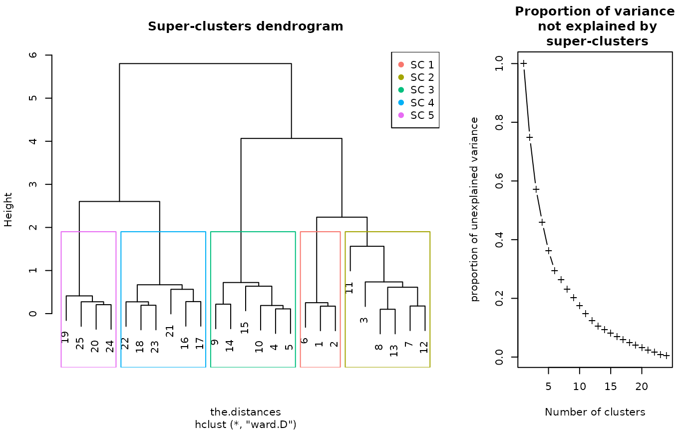
plot(sc.mis, what = "prototypes", type = "grid")## Warning: Using `size` aesthetic for lines was deprecated in ggplot2 3.4.0.
## ℹ Please use `linewidth` instead.
## ℹ The deprecated feature was likely used in the SOMbrero package.
## Please report the issue at <https://github.com/tuxette/SOMbrero/issues>.
## This warning is displayed once every 8 hours.
## Call `lifecycle::last_lifecycle_warnings()` to see where this warning was
## generated.
plot(sc.mis, what = "prototypes", type = "lines")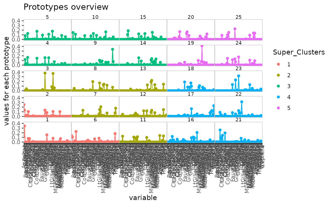
plot(sc.mis, what = "prototypes", type = "mds")
plot(sc.mis, type = "dendro3d")
plot(lesmis, vertex.size = 0,
     vertex.label.color = rainbow(5)[sc.mis$cluster[mis.som$clustering]])
legend(x = "left", legend = paste("SC", 1:5), col = rainbow(5), pch = 19)
cluster 1 contains
Myrieland the characters involved in his sub-story;cluster 2 contains
Valjeanwhich has a central position in the graph visualization, and most of the important character of the novel (including Javert, Fantine and Cosette);cluster 3 contains people almost only connected to
Fantinewho links them to the rest of the novel;cluster 4 contains
Gavroche, the abandoned child of theThenardier, and the characters of his sub-story (including Mr Thénardier and Gavroche’s two brothers and his sister,Eponine);cluster 5 is a bit harder to interpret, with secondary characters related to
Thenardierand to the main characters of the novel.
SOMbrero also contains functions to compute a projected graph based on the super-clusters and to display it:
projectIGraph(sc.mis, lesmis)## IGRAPH 2343a68 UNW- 5 7 --
## + attr: layout (g/n), name (v/c), size (v/n), weight (e/n)
## + edges from 2343a68 (vertex names):
## [1] 1--2 1--3 1--4 2--3 2--4 3--4 4--5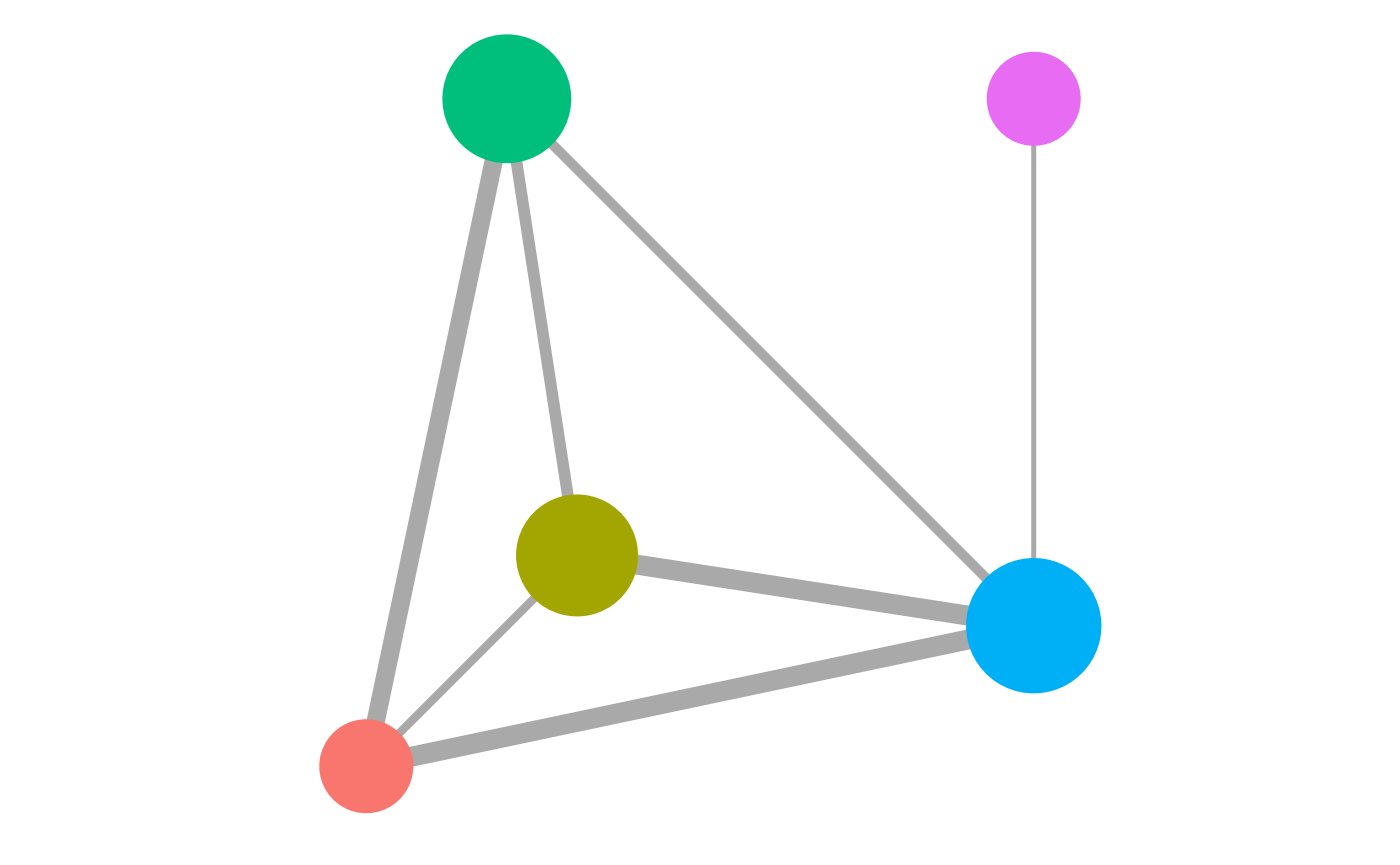
This representation provides a simplified and interpretable display of the graph where the super clusters are represented by nodes with sizes proportional to the number of characters classified in them. The nodes are positioned at the center of gravity of the map clusters included in each super cluster. They are linked to each other with edges with width proportional to the total number of links between two characters of the corresponding super clusters. Here, the central brown/green node is the one of Valjean and the other main characters (super cluster 2), which appears to be strongly related to super cluster 4 in blue, with Gavroche’s neighbors.
Session information
This vignette has been compiled with the following environment:
## R version 4.5.1 (2025-06-13)
## Platform: x86_64-pc-linux-gnu
## Running under: Ubuntu 24.04.3 LTS
##
## Matrix products: default
## BLAS:   /usr/lib/x86_64-linux-gnu/openblas-pthread/libblas.so.3
## LAPACK: /usr/lib/x86_64-linux-gnu/openblas-pthread/libopenblasp-r0.3.26.so;  LAPACK version 3.12.0
##
## locale:
##  [1] LC_CTYPE=en_US.UTF-8       LC_NUMERIC=C
##  [3] LC_TIME=fr_FR.UTF-8        LC_COLLATE=en_US.UTF-8
##  [5] LC_MONETARY=fr_FR.UTF-8    LC_MESSAGES=en_US.UTF-8
##  [7] LC_PAPER=fr_FR.UTF-8       LC_NAME=C
##  [9] LC_ADDRESS=C               LC_TELEPHONE=C
## [11] LC_MEASUREMENT=fr_FR.UTF-8 LC_IDENTIFICATION=C
##
## time zone: Europe/Paris
## tzcode source: system (glibc)
##
## attached base packages:
## [1] stats     graphics  grDevices utils     datasets  methods   base
##
## other attached packages:
## [1] SOMbrero_1.5.0 markdown_2.0   igraph_2.1.4   ggplot2_4.0.0
##
## loaded via a namespace (and not attached):
##  [1] sass_0.4.10          generics_0.1.4       xml2_1.4.0
##  [4] stringi_1.8.7        digest_0.6.37        magrittr_2.0.4
##  [7] evaluate_1.0.5       grid_4.5.1           RColorBrewer_1.1-3
## [10] fastmap_1.2.0        plyr_1.8.9           jsonlite_2.0.0
## [13] backports_1.5.0      ggwordcloud_0.6.2    scales_1.4.0
## [16] isoband_0.2.7        textshaping_1.0.3    jquerylib_0.1.4
## [19] cli_3.6.5            crayon_1.5.3         rlang_1.1.6
## [22] scatterplot3d_0.3-44 litedown_0.7         commonmark_2.0.0
## [25] withr_3.0.2          cachem_1.1.0         yaml_2.3.10
## [28] tools_4.5.1          deldir_2.0-4         memoise_2.0.1
## [31] checkmate_2.3.3      dplyr_1.1.4          colorspace_2.1-2
## [34] interp_1.1-6         vctrs_0.6.5          R6_2.6.1
## [37] png_0.1-8            lifecycle_1.0.4      stringr_1.5.2
## [40] fs_1.6.6             htmlwidgets_1.6.4    ragg_1.5.0
## [43] pkgconfig_2.0.3      desc_1.4.3           pkgdown_2.1.3
## [46] pillar_1.11.1        bslib_0.9.0          gtable_0.3.6
## [49] glue_1.8.0           data.table_1.17.8    Rcpp_1.1.0
## [52] systemfonts_1.3.1    xfun_0.53            tibble_3.3.0
## [55] tidyselect_1.2.1     knitr_1.50           farver_2.1.2
## [58] htmltools_0.5.8.1    labeling_0.4.3       rmarkdown_2.30
## [61] metR_0.18.2          compiler_4.5.1       S7_0.2.0
## [64] gridtext_0.1.5